Recurrence, Recursion and Iterations

The author discusses the differences and relationships between these there important concepts.

If any readers had read the popular fiction the Da Vinci Code, they would remember its gruesome start. They could be excused to have forgotten the anagram  of numbers written on the floor of Le Louvre. This sequence of numbers was immortalised by the victim of a gruesome assassination with his own blood. Perhaps they would have remembered how the main character, Professor Langdon, solves the anagram to form the sequence “1,1,2,3,5,8,13,21″. This sequence of numbers not only plays an important role in this gripping thriller, but it is in fact much older. It originated from India and was formalised by Leonardo of Pisa (also known as Fibonacci) during the medieval period, by  equation 1.

. (1)

 (2)

The Fibonacci numbers are not the only sequence that grows large very quickly, Lucas numbers  are defined with a similar equation (see equation 2). These two sequences can form a beautiful spiral. Like magic, the Fibonacci numbers can also be obtained with the sum of the shallow diagonals of a the Pascal’s triangle. Such behaviour becomes useful model many biological settings, such as the fruitlets of a pineapple or even the arrangement of a pine cone.

 Fig. 1 The Fibonacci numbers and the Pascal’s Triangle

Recurrent relation and the evolution

The Fibonacci numbers and the Lucas numbers rely on previous elements (i.e n-1 and n-2) of the series to compute the current number  n. These are referred as recurrent relation. Now if we imagine our family tree though time, the number of individuals varies. We are all the product of a method of reproduction (natural or in vitro). If our circumstances, experiences and genetic code give us the tools to survive in a given environment, then we are likely to reproduce healthy offsprings; those will increase our family.  At a certain moment in time, every individual will cease to live reducing sadly the size of our family.  So it is feasible to represent mathematically such evolution with two formulae:

gen  = survive(reproduction(select(gen-1))) (3)

gen  = survive(experience(reproduction(select(gen-1)))) (4)

These formulae demonstrate a generation of a family is dependent on the previous one, for their genetic code, but both represent two interesting and different ideas about natural evolution.  In the first expression, Darwinism is represented as only the genetic make-up is taken into account. This theory suggests that inherited variation the genetic code can increase the individual’s abilities to compete, reproduce and survive. Through times species adapt to their environment and some new ones can arise. The second representation take into account our experiences and how they are likely to affect positively or negatively our probability to survive in the present. Lamarckism extend the Darwinism by suggesting characteristics acquired during our lifetime can be passed on to our offspring. It comes to mind that our offsprings are likely to have a better start in life, if we have some sort of financial security or even better if we are wealthy.

These ideas form the premises of evolutionary algorithms.  These non-deterministic algorithms search for good solutions of a problem in the solution search space. This set represents every possible solution, and consequently can be split in smaller sub-sets; some of them will hold better solutions than others. You must be wondering how evolutionary algorithms can tell whether a solution is a good one. Well it works by testing the solution; if the solution meets a set of well-defined criteria, then it will receive a good mark. This type of fitness evaluation mimics Charles Darwin idea, that only the best individuals survive and may pass their genes to the next generation.

Similarly to nature, these algorithms take advantage of probability to generate and reproduce. The reproduction process combines genes from two selected individuals, so that their genetic make-up pass through generations and keep the genes pool varied.

A method to compute recurrent relations

Mathematically these recurrent relations can occur until infinity.

• Let’s imagine that an element of the Fibonacci numbers as an index n, then as the sequence is generated the index the elements becomes large, moving towards infinity. n would then be defined as {n is an integer, where 0 <= n}<= infinity}. 
• The elements of the Pascal Triangle are referred with a row n and a column k. As the triangle grows, both values of k and n increases too. Their values tend to infinity.
• Within an evolution, the number of generation increases too through time. From our ancestors living in prehistoric time, many generations of individuals are born, have lived, perhaps reproduced before dying. This number of generation is continually increasing moving towards infinity. So, it is feasible to define generations as  {generation is an integer, where 0 <= generation <= infinity}.

In these three examples, some common characteristics can be identified. Information is retrieved from previous elements as an input and then transformed to create a new one. All of these objects are of the same type; i.e. a number or an individual of a specie. Secondly, the same series of operations, albeit being just one mathematical operator, are repetitively applied. For the deterministic sequences, a pattern should arise. Finally, each element of these recurrent relations is uniquely identify by a unique identifier (i.e. an index or a generation).

So how can these recurrent relations be computed with a method that can be simply expressed, easily applied and promote re-use of operations. Recursion is one powerful mechanism satisfies these important criteria.  It is a method uses again its own definition. All the recursive methods below use again their definition of the function within their definition.  All of them have a base that starts the sequence.

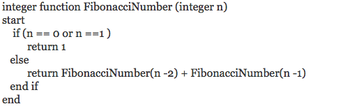
The recursive method for calculating the Fibonacci Numbers

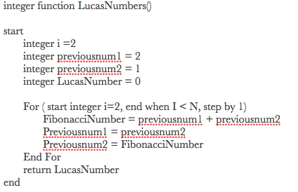
The recursive method for calculating the Lucas Numbers

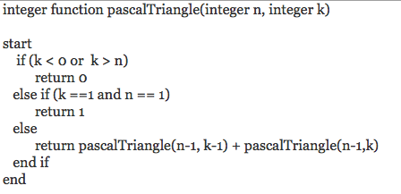
The recursive method for calculating the Pascal’s Triangle

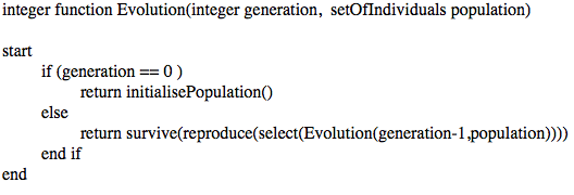
The recursive method for modelling the evolution

Recursion in  computer science

Mathematicians are at ease with such definition, but a computer scientist may not share this opinion. The formal definition of a Turing machine includes a function F that halts the process. Turing machines have modelled theoretically computers since the 1930s and computer science has developed with Turing machines in mind. Based on this idea, infinity has a limit; in Java 1.7 * 10^308 is often consider as the positive largest number. Nonetheless, the concept of recursion is one of the central ideas of computer science. A computer scientist would write these recursive methods differently, using a « tail » method.  In such recursion, the function starts with the largest value of n, and then stop when n = 0 or reach the first base.

   

Spam, Spam, Spam…

The Monty Python sketch has not only named the method to send unsolicited emails, but can also introduce our second and last method. In this short humourous story, the same word is repeated over and over again. The reader can guess which one by the tittle…

Iteration repeats the same actions until a certain condition is met. Programming languages tend to include two types.

• A while loop only stops when a condition is not met. For example, in  the second implementation of the function FibonacciNumber, the while loop terminates if and only if when the value of i becomes equal to the value of N.
• A for loop constantly increments a the value of a variable with a constant until it reaches a limit; if this constant is negative then the values decrease towards their values. In the implementation of the LucasNumber function, a for loop starts with an initial value of 2, then increases the value of i by 1, until it is equal to the value of the constant N.

 

 

The real power of iterations

Recursion works well with any circumstances in which its own definition can be used again. This method suitably produces short and simple mathematical functions and computer programs, for recurrent relations. These implementations rely on at least one base element a selection (i. e. if statement) to decide whether to call its own definition or a base case to stop. This type of programs can be efficient, but can stop working when the random access memory is fully used.

implementing of recurrent relations with an iteration has the major drawback of adding unnecessary complexity to the code. This is specially true in computer science. However, less random access memory is used and the call stack is prevented to overflow. These are the compromises to do, when physically implementing recurrent relations. This second method uses a condition to stop iterating, which can be more flexible than stopping once a base case is reached. When reading, an XML file the only indicator that the end of the file has been read is provided by a function called endOfFile. The end of file can be the second line or the one thousandth  line; it is unknown as it varies with the size of the file. With a while loop, this unique function can read the whole file without worrying the number of lines; it is a more general statement.

Conclusion

We have discussed and explain the relationship between Recurrence, Recursion and Iterations. Recurrence can be either be implemented by an iterations or a recursion. As soon as a stopping criterion becomes more complex than a simple equality or inequality, an iteration offers a better option. In our next post the author will explore further the non-deterministic evolutionary algorithms.